Week 9 - Driven Oscillators and Resonance¶

Thus far, we have either worked with energy conserving systems or systems that dissipate energy to the point of stopping their motion. The primary examples have been conservative systems, potential energy oscillators, and systems with damping that extract all the kinetic energy from the system. Driven Systems are systems that are driven by external forcing. We use "forcing" because it's not always a push or a pull. Radio systems use electromagnetic waves to drive the system. Climate systems are driven by thermal forcing.

Driven oscillators are a specific type of driven system, we expect them to demonstrate recurrent bahevior. Driven ooscillators are quite common. Analog radios use a driven oscillator that is tuned to a specific frequency (99.5 FM is tuned to 99.5 MHz). When you dial the radio you are "tuning" the oscillator to the frequency of the broadcast. This is an illustration of the phenomenon of resonance. Resonance is a phenomenon where a system is driven at a frequency that matches (or closely matches) its natural frequency. When this happens, the amplitude of the oscillation can grow very large. Resonance is the phenomenon that caused the collapse of the Tacoma Narrows Bridge) in 1940.

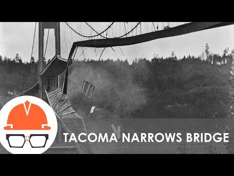
Collapse of the Tacoma Narrows Bridge (9 minute video)¶

Resonance is the phenomenon that caused the collapse of the Tacoma Narrows Bridge) in 1940. The video below describes the collapse and how the bridge was rebuilt to avoid the same problem.

Quantum Mechanical Resonance¶

You might have heard about resonance in the context of quantum mechanics) or most likely in particle physics or nuclear physics. In these cases, typically resonance is a phenomenon where a system is driven at a frequency that matches some natural spacing of energy levels. In quantum mechanics, frequency of light is related to it's energy by $E = h \nu$, where $h$ is Planck's constant and $\nu$ is the frequency of the light.

The energy levels of a system are quantized, they are separated by discrete amounts. When a system is driven at a frequency that matches the energy level separation, the system can absorb energy from the driving force. This can cause the system to transition to a higher energy state. A quantum system also ejects an amount of energy as a photon (randomly) and transitions to a lower energy state.

Probing these transitions can tell you about particle properties and reactions. This is a large field of study in particle and nuclear physics.

Solving Linear Differential Equations¶

Much of the work we have done so far has been solving homogeneous linear differential equations. These are equations that have a form like this:

$$\frac{d^2 x}{dt^2} + 2\beta\frac{dx}{dt} + \omega_0^2 x = 0.$$

All of the driven systems that we will work with will be described by a linear differential equation. The general form of a linear differential equation is:

$$\frac{d^n x}{dt^n} + a_{n-1} \frac{d^{n-1} x}{dt^{n-1}} + a_{n-2} \frac{d^{n-2} x}{dt^{n-2}} + ... + a_1 \frac{dx}{dt} + a_0 x = f(t).$$

The $f(t)$ is the driving force. The $a_i$ are constants. The $n$ is the order of the differential equation.

We've never solved a driven differential equation before, but we have two powerful tools: superposition and uniqueness. Superposition tells us that we can solve the homogeneous part of the equation and then add a particular solution to get the full solution. Uniqueness tells us that if we have a solution that fits the driver and the initial conditions, then it is unique.

As the homogenous solutions for our oscillators will typically die out, we will refer to them as transient solutions. The particular solution will be the steady state solution.